# Evaluation Metrics for Classifier that Every Machine Learning Engineer Should Know
## Preface
Recently I've to complete the machine learning life cycle on my previous project which have applied the binary classifier.
As we finished to build the prototype of machine learning model in first stage, the second stage is to take the maintainability
into the consideration.
How we decide to deploy to use a new model? What metrics should we take care under the current circumstance
is important for the every machine learning engineer.
## Binary Classification
### What's the binary classification?
The input of the binary classification can be either numerical value or the categorical encoded value and the output is an one dimensional value within [0, 1].
### When do we apply binary classification?
The best practice to implement the binary classification is in the occasion of yes or no case.
## Type of the Metrics
Before to introduce the classification metrics, there are the things you should know.
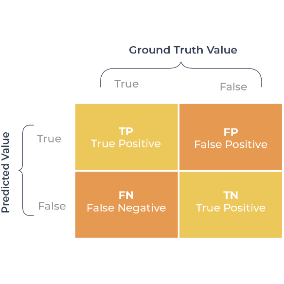
* TP: The model predict with positive result which is ground truth positive
* FP: The model predict with positive result which is ground truth negative
* TN: The model predict with negative result which is ground truth negative
* FN: The model predict with negative result which is ground truth positive
The 4 types of the prediction results can be form into the confusion matrix
https://arize.com/glossary/confusion-matrix/
After known the 4 types of predictions, we can start to learn the evaluation metrics
### Accuracy
$$ \dfrac{TP + TN}{TP + TN + FP + FN} $$
> **_Semantic_**: Take both positive and negative cases into account to evaluate the
quality of the classification
{{< admonition note "Implementation" >}}
```python
from sklearn.metrics import accuracy_score
prediction = [0, 1, 0, 1]
ground_truth = [0, 1, 1, 1]
score = accuracy_score(prediction, ground_truth)
```
{{< /admonition>}}
### Precision
$$ \dfrac{TP}{TP + FP} $$
> **_Semantic_**: Focus on the correct ratio which model predict is positive is ground truth positive.
{{< admonition note "Implementation" >}}
```python
from sklearn.metrics import precision_score
prediction = [0, 1, 0, 1]
ground_truth = [0, 1, 1, 1]
score = precision_score(prediction, ground_truth)
```
{{< /admonition>}}
### Recall
$$ \dfrac{TP}{TP + FN} $$
> **_Semantic_**: Focus on the ratio of the ground truth positive label which model is predict to the positive.
{{< admonition note "Implementation" >}}
```python
from sklearn.metrics import recall_score
prediction = [0, 1, 0, 1]
ground_truth = [0, 1, 1, 1]
score = recall_score(prediction, ground_truth)
```
{{< /admonition>}}
### F1-score
$$ 2 \cdot \dfrac{Precision \cdot Recall}{Precision + Recall} $$
> **_Semantic_**: The harmonic mean of precision and recall on the model predict positive side.
{{< admonition note "Implementation" >}}
```python
from sklearn.metrics import f1_score
prediction = [0, 1, 0, 1]
ground_truth = [0, 1, 1, 1]
score = f1_score(prediction, ground_truth)
```
{{< /admonition>}}
### AUROC
> **_Semantic_**: The area under ROC(which will introduce later), the score is within the interval [0, 1].
AUROC shows the ability of the classifier to separate the outcome prediction score, the larger AUROC the
model has, the better the model perform.
## How to evaluate the model with the metrics?
### Check confusion matrix first
Imagine if we are in the condition that we have TP=100, TN=1, FP=1, FN=10. Under
this circumstance if we choose accuracy as the metric in advance, the result will
show that if we set the model to predict with positive result no matter what's the
coming input, it still can give us a good performance. In this case, watching the
accuracy may be not so meaningful for us.
### Which side of the prediction we more care about?
After we have checked the confusion matrix and accuracy, we can move on to select
positive or negative outcome we care about, and compute the precision and recall
base on the side we want to observe. Evaluate F1-score is a good way to take both
precision and recall into the consideration.
## Optimize the Classification Threshold
There's problem that we may be encounter, if the model outcome distribution is different
between training and testing (production), how could we modify the classification threshold?
Or maybe we are training the data one the NN model which the last layer output by a softmax
function, how could we choose the prediction threshold?
### PR-curve
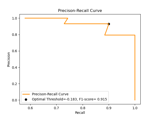
> **_Property_**: To show the relation between precision and recall by moving the the
threshold to the different place iteratively. As the recall become larger, the precision would be smaller.
We can find the threshold has the largest F1-score, which the threshold is
optimal for positive or negative side.
{{< admonition note "Implementation" >}}
```python
import matplotlib.pyplot as plt
import numpy as np
from sklearn.datasets import load_iris
from sklearn.model_selection import train_test_split
from sklearn.pipeline import make_pipeline
from sklearn.preprocessing import StandardScaler
from sklearn.svm import LinearSVC
from sklearn.metrics import precision_recall_curve
X, Y = load_iris(return_X_y=True)
# Add noisy features
random_state = np.random.RandomState(0)
n_samples, n_features = X.shape
X = np.concatenate([X, random_state.randn(n_samples, 100 * n_features)], axis=1)
# Limit to the two first classes, and split into training and test
X_train, X_test, Y_train, Y_test = train_test_split(
X[Y < 2], Y[Y < 2], test_size=0.5
)
classifier = make_pipeline(StandardScaler(), LinearSVC())
classifier.fit(X_train, Y_train)
# PR-curve
Y_pred_score = classifier.decision_function(X_test)
precisions, recalls, thresholds = precision_recall_curve(Y_test, Y_pred_score)
# Find optimized threshold
f1_scores = (2 * precisions * recalls) / (precisions + recalls)
optimal_threshold_idx = np.argmax(f1_scores)
optimal_threshold = float(thresholds[optimal_threshold_idx])
# Show result
fig = plt.figure()
line_width = 2
plt.plot(precisions, recalls, color="darkorange", lw=line_width, label="Precison-Recall Curve")
plt.scatter(
precisions[optimal_threshold_idx],
recalls[optimal_threshold_idx],
marker="o",
color="black",
label=f"Optimal Threshold={optimal_threshold: .3f}"
+ f", F1-score={f1_scores[optimal_threshold_idx]: .3f}"
)
plt.xlabel("Recall")
plt.ylabel("Precision")
plt.title("Precison-Recall Curve")
plt.legend(loc="best")
```
{{< /admonition>}}
### ROC
At the previous section we have talked about AUROC, which is calculate the area under the curve.
Before we start to dive in to ROC, first I want to introduce two metrics
* TP rate: $$ \dfrac{TP}{TP + FN} = Recall $$
* FP rate: $$ \dfrac{FP}{FP + TN} $$
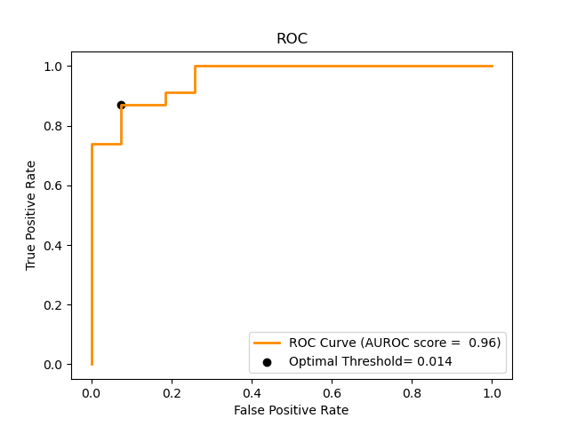
> **_Property_**: To show the relation between TP rate and FP rate by moving the the
threshold to the different place iteratively. As the TP rate become larger, the FP rate would be larger.
We can find the threshold has the largest g-means, which is the optimal threshold
for separating the outcome distribution.
* g-means: $$ \sqrt{TP rate \cdot (1 - FP rate)} $$
{{< admonition note "Implementation" >}}
```python
import matplotlib.pyplot as plt
import numpy as np
from sklearn.datasets import load_iris
from sklearn.model_selection import train_test_split
from sklearn.pipeline import make_pipeline
from sklearn.preprocessing import StandardScaler
from sklearn.svm import LinearSVC
from sklearn.metrics import roc_curve, roc_auc_score
X, Y = load_iris(return_X_y=True)
# Add noisy features
random_state = np.random.RandomState(0)
n_samples, n_features = X.shape
X = np.concatenate([X, random_state.randn(n_samples, 100 * n_features)], axis=1)
# Limit to the two first classes, and split into training and test
X_train, X_test, Y_train, Y_test = train_test_split(
X[Y < 2], Y[Y < 2], test_size=0.5
)
classifier = make_pipeline(StandardScaler(), LinearSVC())
classifier.fit(X_train, Y_train)
# ROC
Y_pred_score = classifier.decision_function(X_test)
auroc_score = roc_auc_score(Y_test, Y_pred_score)
fp_rate, tp_rate, thresholds = roc_curve(Y_test, Y_pred_score)
# Find optimized threshold
gmeans = np.sqrt(tp_rate * (1 - fp_rate))
optimal_threshold_idx = np.argmax(gmeans)
optimal_threshold = float(thresholds[optimal_threshold_idx])
# Show result
fig = plt.figure()
line_width = 2
plt.plot(
fp_rate,
tp_rate,
color="darkorange",
lw=line_width,
label=f"ROC Curve (AUROC score = {auroc_score: .2f})",
)
plt.scatter(
fp_rate[optimal_threshold_idx],
tp_rate[optimal_threshold_idx],
marker="o",
color="black",
label=f"Optimal Threshold={optimal_threshold: .3f}"
)
plt.xlabel("False Positive Rate")
plt.ylabel("True Positive Rate")
plt.title("ROC")
plt.legend(loc="best")
```
{{< /admonition>}}
## Conclusion
Using right way to evaluate the classifier is important.
* Knowing the distribution of the ground truth label give us the confidence to using accuracy.
* Use Precision, Recall, F1-score to evaluate the model if you're more care about
the performance on the positive or negative side for your use case.
* Optimize the classifier threshold for your use case.
## Reference
[1] Scikit-learn - https://scikit-learn.org/stable/auto_examples/model_selection/plot_precision_recall.html#precision-recall
 {{< /admonition>}}
### ROC
At the previous section we have talked about AUROC, which is calculate the area under the curve.
Before we start to dive in to ROC, first I want to introduce two metrics
* TP rate: $$ \dfrac{TP}{TP + FN} = Recall $$
* FP rate: $$ \dfrac{FP}{FP + TN} $$
> **_Property_**: To show the relation between TP rate and FP rate by moving the the
threshold to the different place iteratively. As the TP rate become larger, the FP rate would be larger.
We can find the threshold has the largest g-means, which is the optimal threshold
for separating the outcome distribution.
* g-means: $$ \sqrt{TP rate \cdot (1 - FP rate)} $$
{{< admonition note "Implementation" >}}
```python
import matplotlib.pyplot as plt
import numpy as np
from sklearn.datasets import load_iris
from sklearn.model_selection import train_test_split
from sklearn.pipeline import make_pipeline
from sklearn.preprocessing import StandardScaler
from sklearn.svm import LinearSVC
from sklearn.metrics import roc_curve, roc_auc_score
X, Y = load_iris(return_X_y=True)
# Add noisy features
random_state = np.random.RandomState(0)
n_samples, n_features = X.shape
X = np.concatenate([X, random_state.randn(n_samples, 100 * n_features)], axis=1)
# Limit to the two first classes, and split into training and test
X_train, X_test, Y_train, Y_test = train_test_split(
X[Y < 2], Y[Y < 2], test_size=0.5
)
classifier = make_pipeline(StandardScaler(), LinearSVC())
classifier.fit(X_train, Y_train)
# ROC
Y_pred_score = classifier.decision_function(X_test)
auroc_score = roc_auc_score(Y_test, Y_pred_score)
fp_rate, tp_rate, thresholds = roc_curve(Y_test, Y_pred_score)
# Find optimized threshold
gmeans = np.sqrt(tp_rate * (1 - fp_rate))
optimal_threshold_idx = np.argmax(gmeans)
optimal_threshold = float(thresholds[optimal_threshold_idx])
# Show result
fig = plt.figure()
line_width = 2
plt.plot(
fp_rate,
tp_rate,
color="darkorange",
lw=line_width,
label=f"ROC Curve (AUROC score = {auroc_score: .2f})",
)
plt.scatter(
fp_rate[optimal_threshold_idx],
tp_rate[optimal_threshold_idx],
marker="o",
color="black",
label=f"Optimal Threshold={optimal_threshold: .3f}"
)
plt.xlabel("False Positive Rate")
plt.ylabel("True Positive Rate")
plt.title("ROC")
plt.legend(loc="best")
```
{{< /admonition>}}
### ROC
At the previous section we have talked about AUROC, which is calculate the area under the curve.
Before we start to dive in to ROC, first I want to introduce two metrics
* TP rate: $$ \dfrac{TP}{TP + FN} = Recall $$
* FP rate: $$ \dfrac{FP}{FP + TN} $$
> **_Property_**: To show the relation between TP rate and FP rate by moving the the
threshold to the different place iteratively. As the TP rate become larger, the FP rate would be larger.
We can find the threshold has the largest g-means, which is the optimal threshold
for separating the outcome distribution.
* g-means: $$ \sqrt{TP rate \cdot (1 - FP rate)} $$
{{< admonition note "Implementation" >}}
```python
import matplotlib.pyplot as plt
import numpy as np
from sklearn.datasets import load_iris
from sklearn.model_selection import train_test_split
from sklearn.pipeline import make_pipeline
from sklearn.preprocessing import StandardScaler
from sklearn.svm import LinearSVC
from sklearn.metrics import roc_curve, roc_auc_score
X, Y = load_iris(return_X_y=True)
# Add noisy features
random_state = np.random.RandomState(0)
n_samples, n_features = X.shape
X = np.concatenate([X, random_state.randn(n_samples, 100 * n_features)], axis=1)
# Limit to the two first classes, and split into training and test
X_train, X_test, Y_train, Y_test = train_test_split(
X[Y < 2], Y[Y < 2], test_size=0.5
)
classifier = make_pipeline(StandardScaler(), LinearSVC())
classifier.fit(X_train, Y_train)
# ROC
Y_pred_score = classifier.decision_function(X_test)
auroc_score = roc_auc_score(Y_test, Y_pred_score)
fp_rate, tp_rate, thresholds = roc_curve(Y_test, Y_pred_score)
# Find optimized threshold
gmeans = np.sqrt(tp_rate * (1 - fp_rate))
optimal_threshold_idx = np.argmax(gmeans)
optimal_threshold = float(thresholds[optimal_threshold_idx])
# Show result
fig = plt.figure()
line_width = 2
plt.plot(
fp_rate,
tp_rate,
color="darkorange",
lw=line_width,
label=f"ROC Curve (AUROC score = {auroc_score: .2f})",
)
plt.scatter(
fp_rate[optimal_threshold_idx],
tp_rate[optimal_threshold_idx],
marker="o",
color="black",
label=f"Optimal Threshold={optimal_threshold: .3f}"
)
plt.xlabel("False Positive Rate")
plt.ylabel("True Positive Rate")
plt.title("ROC")
plt.legend(loc="best")
```
 {{< /admonition>}}
## Conclusion
Using right way to evaluate the classifier is important.
* Knowing the distribution of the ground truth label give us the confidence to using accuracy.
* Use Precision, Recall, F1-score to evaluate the model if you're more care about
the performance on the positive or negative side for your use case.
* Optimize the classifier threshold for your use case.
## Reference
[1] Scikit-learn - https://scikit-learn.org/stable/auto_examples/model_selection/plot_precision_recall.html#precision-recall
{{< /admonition>}}
## Conclusion
Using right way to evaluate the classifier is important.
* Knowing the distribution of the ground truth label give us the confidence to using accuracy.
* Use Precision, Recall, F1-score to evaluate the model if you're more care about
the performance on the positive or negative side for your use case.
* Optimize the classifier threshold for your use case.
## Reference
[1] Scikit-learn - https://scikit-learn.org/stable/auto_examples/model_selection/plot_precision_recall.html#precision-recall